 VoltSim
Plot your first waveform
A waveform is a picture of a signal changing over time. A trace is the colored line for that signal, and a channel is one of the scope’s four places to plot a trace.
- Open a circuit with a changing signal. To make a simple one, place an AC Voltage source, connect its negative terminal to Ground, and set it to a 100 Hz sine wave with a 2 V peak and zero bias.
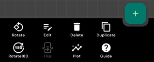
- Select the source and choose Plot. Look for Plot in the component toolbar or its More menu. In Parameters to display, select Voltage (V) and confirm with Plot.
- Tap Run. The scope opens when you add a signal. Give the trace time to fill the plot. Use the graph icon in the simulator toolbar (Toggle Oscilloscope) to reopen the panel if you close it.
Repeat with another component to compare signals. Each quantity you plot uses one channel. For the voltage at a node relative to circuit ground, connect a Probe and leave its type set to Voltage. A two-terminal component generally plots the voltage across its terminals. The available choices depend on the component.
Read the grid
- Across the screen
- In Time view, each horizontal grid division represents an amount of simulated time. Newest samples appear on the right. At 2 ms/div, five divisions span 10 ms.
- Up and down the screen
- The vertical axis shows the value and its unit, such as volts (V) or milliamps (mA). At 1 V/div, a signal spanning four divisions from bottom to top swings by 4 V peak-to-peak.
- One complete cycle
- Measure from one peak to the next, or from one rising edge to the next. That interval is the period. Frequency is 1 divided by the period in seconds, so a period of 10 ms (0.010 s) is 100 Hz.
For the 100 Hz practice signal, expect a crest near +2 V and a trough near −2 V. The full swing is 4 V peak-to-peak.
Time scale, time step, and speed
Use Horizontal Scale to frame the signal, Time Step to change how finely the circuit is calculated, and Speed to make the live simulation easier to watch.
Horizontal Scale controls the time axis
Open Settings Bar → Horizontal → Time. Move Horizontal Scale left for less simulated time per division and more detail on an edge. Move it right to show more cycles or a longer event. The scope groups more simulator steps into each plotted sample as you move right, so short pulses can become harder to see. The circuit keeps using the same time step.
Enable Gesture in the Horizontal tab to swipe left to zoom in or right to zoom out. Swiping changes how much of the capture is visible while keeping the sample spacing and time per division. For timestamps along the bottom, enable Show Time Labels under Settings Bar → General → Settings → Time.
Time Step controls the solver’s detail
Open the simulator’s main menu (☰), expand Simulation Setting, and choose Time Step. Enter a value and confirm. A smaller step calculates the circuit at shorter intervals, which helps resolve fast signals and makes smaller time scales available. The extra calculations can make the simulation take longer. A larger step covers more simulated time per calculation, but it can miss fast edges or make a fast signal appear at the wrong frequency.
Start with the scale slider. If its smallest scale is still too coarse, reduce the time step. The dialog estimates the highest source frequency that the step can resolve, and setting a faster source can lower the step automatically. Changing Time Step resets simulated time to zero and clears the scope history. Let the simulation run to fill the plot again.
Speed controls how fast the simulation runs
Move Speed left to slow down a switching event as you watch it, or right to reach steady behavior sooner. The slider in the scope’s Horizontal tab and the one under Simulation Setting control the same setting. A 100 Hz signal still takes 10 ms of simulated time per cycle at any speed. Use Hold when you want to freeze just the trace.
Enable Show Stats in Simulation Setting to compare Set speed with Real speed. A ratio of 1:10 means one simulated second takes about ten seconds on the clock. A small time step or a circuit with more work to do can slow progress. Current display speed only changes the animation of current indicators.
Try it with the 100 Hz wave. In the waveform diagram, go from 2 ms/div to 5 ms/div. One 10 ms cycle goes from five divisions to two. In the app, try lowering Speed and watch the same 10 ms cycle scroll more slowly. Then keep the scale slider in place and change Time Step from 5 µs to 2.5 µs. The scope’s sample spacing halves, and the solver takes about twice as many steps to cover the same 10 ms.
Vertical scale and channels
Set the height and position
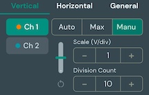
In Vertical, choose a channel and pick a scale mode.
- Auto
- Fits the range to the signal. Auto channels with the same unit share a scale so you can compare their heights. Start here if you lose a trace.
- Max
- Sets symmetric limits around zero. Enter 5 V to set the range from −5 V to +5 V.
- Manual
- Set the units per division, the division count, and the vertical offset. Use the offset slider to reposition the trace and the reset arrow to center the scale on zero. Division Count applies across channels.
Organize several channels
- Hide or Show a trace with its color swatch in the readouts or the eye button in Vertical. A hidden channel still occupies its slot.
- Invert flips the direction of a channel’s vertical axis. It changes how the graph is drawn.
- Remove frees one slot. The scope bar’s Clear All removes every plotted channel.
- Split overlapping traces by swiping down on the graph. Swipe up to overlay them again. Enable Vertical Swipe under Settings → Gestures if needed.
Measure a signal
Tap the readouts beneath the plot to expand them into a table for all plotted channels. For a stable repeating signal, give the plot time to fill with several cycles.

- Max and Min
- The highest and lowest measured values. Subtract Min from Max for the peak-to-peak swing.
- Freq
- How many times the waveform repeats each second. A steady DC value or a signal without a consistent period may have a blank frequency.
- RMS
- Root mean square, the effective size of a signal. A zero-bias sine wave with a 2 V peak reads about 1.41 V RMS over complete cycles.
Read a point or a range
In the Settings Bar’s General tab, turn on one of these tools.
- Hold freezes the displayed traces while the circuit keeps running. Turn Hold off to see the live traces again.
- Cursor places a vertical line on the plot. Drag from near the line. In Time view, it shows the time and each visible trace’s value. In Spectrum view, it shows the frequency and each trace’s amplitude or dB level.
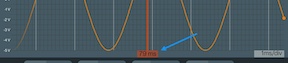
- Measure adds two vertical markers in Time view. Drag each marker to a boundary. The label between them shows the elapsed time, and the readouts use the selected interval. Turn Measure off to return to the full visible time window.
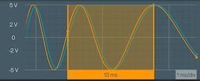
Try it. Turn on Hold, then Measure. Align the two markers with adjacent peaks of the 100 Hz sine wave and look for about 10 ms between them. To check RMS or automatic frequency, widen the interval to include several complete cycles.
The scope scrolls freely. Trigger Mode is shown as None, so a repeating trace can drift across the screen while the simulation runs.
Compare gain and phase
Use this when you send a steady sine wave into a filter or amplifier and want to see how the circuit changes it. Plot the input and output as separate channels.
- Open Settings Bar → General. Under Gain / phase reference, select the input channel.
- Expand the readouts below the graph. Each other channel is compared with the reference at the reference’s fundamental frequency, the frequency of its repeating sine wave.
- Use the full visible window or choose a steady interval with Measure. Include at least two complete cycles with enough samples per cycle. Tap the selected reference again to switch the comparison off.
- Gain
- The response amplitude divided by the reference amplitude. A gain of 0.5 means the response is half the input amplitude.
- dB
- Gain expressed in decibels. For channels with matching units, 0 dB means equal amplitudes, and half amplitude is about −6 dB. If the units differ, gain carries a unit such as mA/V and the dB cell is blank.
- Phase
- How far the response is ahead of or behind the reference within a cycle. Positive means it leads. Negative means it lags. A quarter-cycle delay is −90°.
Try it. Make an RC low-pass filter from the practice circuit. Connect a 1 kΩ resistor from the source’s positive terminal to a new output node, then connect a 1 µF capacitor from that node to ground. Plot the source voltage and a Probe on the output node. Set the source to 159 Hz, near the filter’s cutoff frequency, and select the source channel as the reference. Expect about 0.707 gain, −3 dB, and −45° phase.
If you see dashes, let the circuit settle, check that both signals are steady sinusoids, then adjust the time window to show a few clean cycles. The reference selection lasts for the current session.
Explore the spectrum
Where Time view shows when a signal changes, Spectrum shows which frequencies are present. The scope uses an FFT (fast Fourier transform) to turn recent samples into a plot of frequency versus amplitude.
- Open Settings Bar → Horizontal and choose Spectrum.
- Let the simulation collect samples. Use Max Frequency to set the right edge of the plot, or tap Auto Set to frame the frequencies that contain most of the signal’s energy.
- In Vertical, choose Linear for amplitudes in the signal’s units or Log to see smaller peaks in decibels. Read the 0 dB reference shown on the plot. Channels with the same unit share that reference.
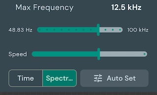
A 100 Hz sine wave gives a main peak near 100 Hz. A square wave also has harmonics, peaks at multiples of its fundamental frequency. A peak at 0 Hz represents a steady offset (DC) when shown in the selected scale.
For nearby peaks, lower Max Frequency while keeping both peaks in view. For higher harmonics, raise it. The upper limit is half the scope’s sample rate in Spectrum mode. Switch back to Time to see individual edges, pulses, or delays.
Choose an acquisition mode
The simulator calculates the circuit in small time steps. When one plotted sample spans several steps, Acquisition Mode determines how those steps appear. Open Settings Bar → General → Settings and use the General tab.
- Sample
- Draws a representative sample with a band showing the low-to-high swing when several steps fit into a plotted sample. A useful starting point for general waveform viewing.
- Average
- Draws the mean of the steps in each sample. Useful for smoothing small fluctuations. Short pulses and spikes can appear smaller.
- Envelope
- Emphasizes the minimum and maximum reached within each sample. Use it to see ripple, brief excursions, or the outline of a fast carrier when individual cycles are too close together.
Sample Rate in the General tab is the number of samples captured per simulated second in the current view. See time scale and time step for how to capture finer detail.
Record and export a capture
- Plot the signals you want and set the capture scale. VoltSim takes the channel list and the time between recorded samples when you start recording.
- With the simulation running, choose Settings Bar → General → Record. Let the event happen, then tap Stop in the scope’s General tab.
- In Export recording, choose Image (.png) for a graph with axes, or File (.csv) for a spreadsheet. Tap Export and pick a destination.
The CSV starts at zero seconds relative to the recording and includes one column per recorded channel, with units in the headings. Changing the display scale mid-recording preserves the starting sample interval. If you remove a recorded channel, its column stops filling. Add any new signals before starting the next recording.
Try it. Record a switch closing. Start recording before tapping the switch, then use the CSV to compare the readings before and after the change.
Display preferences and gestures
Use Settings Bar → General → Settings to open Preferences.
- General
- Use Large Display for a taller plot and Show Cursor to show the movable marker. Digital Mode draws stepped transitions for logic signals. Time Mode and Acquisition Mode select the plot type and sample display.
- Channels
- The General subtab controls the value grid and value labels. Select a channel to set its visibility, line thickness, transparency, or color.
- Time
- Show the time grid and time labels, or adjust the horizontal scale.
- Gestures
- Double Tap switches between normal and large display. Horizontal Swipe zooms the time axis and can also be enabled with Gesture in the Horizontal tab. Vertical Swipe splits or overlays channels.
Troubleshooting
The plot is empty
Confirm that at least one quantity is checked in the component’s Plot dialog. Tap Run, turn off Hold, and make sure the channel is visible. If all four slots are filled, remove a channel and try plotting again.
The signal looks flat, clipped, or crowded
Choose Auto in Vertical and check your probe’s connection. A constant voltage appears as a flat line. In Time view, use less time per division to spread out a crowded signal or more time per division to watch a slow change. Split the channels when traces overlap.
The frequency or phase is blank
Wait for the circuit to settle and widen the range so it contains several complete cycles. Check for a reference channel if you’re measuring gain and phase. A constant signal has no repeating cycle, and an irregular or strongly distorted signal may leave these readouts blank.
The spectrum is empty or the peak is missing
Let several cycles accumulate, check that the channel is visible, then try Auto Set. If you know the expected frequency, set Max Frequency above it. Use Log to inspect weak peaks next to strong ones.
Stop did not open the export dialog
Make sure the simulation is advancing and a signal is plotted before you tap Record. Run long enough for at least one sample, then tap Stop in the scope’s General tab.